Fast Regression Models

Functions to do fast regression modelling. The functions return a tibble with statistics. Use plot() for an extensive model visualisation.

regression(x, ...)

# S3 method for default
regression(x, y = NULL, type = "lm", family = stats::gaussian, ...)

# S3 method for data.frame
regression(x, var1, var2 = NULL, type = "lm", family = stats::gaussian, ...)

# S3 method for certestats_reg
plot(x, ...)

# S3 method for certestats_reg
autoplot(object, ...)

Arguments

x

vector of values, or a data.frame

...

arguments for lm() or glm()

y

vector of values, optional

type

type of function to use, can be "lm" or "glm"

family

only used for glm()

var1, var2

column to use of x, the var2 argument is optional

object

data to plot

Examples

runif(10) |> regression()
#> # A tibble: 2 × 5
#>   term        estimate std.error statistic p.value
#> * <chr>          <dbl>     <dbl>     <dbl>   <dbl>
#> 1 (Intercept)     8.66      2.14      4.06 0.00366
#> 2 x              -5.32      3.27     -1.62 0.143  

data.frame(x = 1:50, y = runif(50)) |>
  regression(x, y)
#> # A tibble: 2 × 5
#>   term         estimate std.error statistic      p.value
#> * <chr>           <dbl>     <dbl>     <dbl>        <dbl>
#> 1 (Intercept)  0.552      0.0806      6.85  0.0000000124
#> 2 x           -0.000727   0.00275    -0.264 0.793       

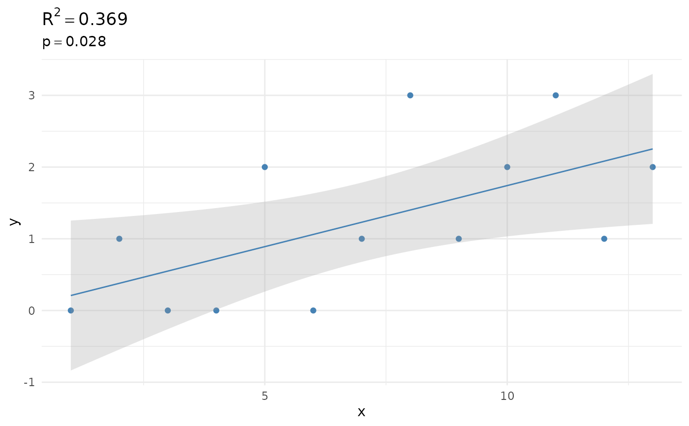
mrsa_from_blood_years <- c(0, 1, 0, 0, 2, 0, 1, 3, 1, 2, 3, 1, 2)
mrsa_from_blood_years |> plot()


mrsa_from_blood_years |> regression()
#> # A tibble: 2 × 5
#>   term        estimate std.error statistic p.value
#> * <chr>          <dbl>     <dbl>     <dbl>   <dbl>
#> 1 (Intercept)     4.33     1.38       3.14 0.00946
#> 2 x               2.17     0.854      2.54 0.0277 

mrsa_from_blood_years |> regression() |> plot()
#> `geom_smooth()` using formula = 'y ~ x'